While optimizing the problem of circular arbitrage opportunity detection, it is best solved by framing the problem as a graph. While learning more about this problem, I wanted to share with you my findings while I was building an FPGA implementation in 2020. Due to confidentiality reasons I cannot share implementation details, but I do wanted to share some of the learnings from that endeavour.

Before we begin, let’s define a graph as a set of nodes (or vertices) and edges. It us up to us to decide what we do with the vertices, edges and weights it represents. If we were to model congestion on a road network, we might say the vertices are junctions, the edges are the roads themselves, and the weights are the average daily congestion of the roads during peak hours.

A typical graph problem is related to finding the shortest path, and there is worth over three centuries of theories and research into this. Ever since Euler started investigating this problem in 1734, it has found many applications, from computer science to economics. As a matter of fact, there exist many efficient algorithms related to finding the shortest path along a graph, which have widespread applications e.g in mapping.

Bellman-Ford

To clarify, this problem has two measures of input size; C is the number of currencies (nodes) and R is the number of exchange rates available (edge weights).

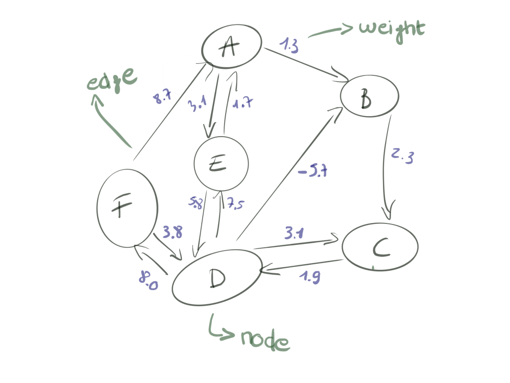
One of these algorithms we will zoom in a bit, is the Bellman-Ford algorithm. This algorithm finds the minimum weight path from a single source vertex to all other vertices on a weighted directed graph. This takes a few iterations with a maximum the total number of verteces minus 1 (|C|-1), where the remarkable feature of the algorithm is that at the end of an iteration, each vertex is labelled with the sum of the minimum weight path from the source to that vertex. Applying this logic to the illustrated network, you will find something strange when calculating the minimum weight path from vertices B to C.

When you are new to graph theory, or Bellman-Ford, you might instinctively say the single-source shortest path is the direct edge between B to C with a weight of 2.3. But because the algorithm is greedy, meaning it will perform multiple iterations, you will notice that actually a shorter (i.e. cheaper) path is actually BCDBC with a total weight of 0.8. If we cycle again, we will be at an even lower weight of -0.7, and so on. In fact, each time we traverse the loop, our minimum total weight will reduce by -1.5.

This is called a negative-weight cycle, the existence of which means that the shortest path between B and C is not defined.

Dijkstra, Floyd-Warshall and Bellman-Ford: Negative-weight cycle in other algorithms

Other shortest path first (SPF) algorithms, such as Dijkstra, are not supporting negative-weight cycles, which we will cover in a minute why this is important for arbitrage trading. Therefore, Dijkstra is not suitable for arbitrage problems.

Another SPF algorithm, Floyd-Warshall, is an equally suited candidate for applying in arbitrage problems, but is an all-pairs-shortest-path algorithm, which means that any of all the nodes can be a source, so you want the shortest distance to reach any destination node from any source node. This only fails when there are negative cycles.

Comparing this to the single-source-shortest-path algorithm of Bellman-Ford, this means that the algorithm works when there is only one single source, and you want to know the shortest path from one node to another.

While both Floyd-Warshall and Bellman-Ford are both dynamic programming algorithms, Floyd-Warshall is not the same algorithm as “for each node v, run Bellman-Ford with v as the source node“. In particular, Floyd-Warshall runs in O(C³), time, while repeated-Bellman-Ford runs in 𝑂(C²R) time, (𝑂(CR) time for each source vertex).

Applying this to currency arbitrage, this means that Bellman-Ford is the best option if you know what base currency you wish to increase. In case you wish to identify opportunities over all currencies that are part as nodes in the graph, then Floyd-Warshall is the better candidate algorithm, however the additional computing logic will most likely suffer your overall arbitrage performance and result in order slippage, and consequently losses.

Performance tweaks of the Bellman-Ford algorithm

While the number of iterations are defined as |V|-1 (total number of nodes minus 1), iterations can be aborted prematurely if after the last iteration no new changes are observed. In large graphs, this will be significantly reduce the computing cost. In this case the worst case of the algorithm remains unchanged.

Applying Bellman-Ford for currency arbitrage

When applying translating an arbitrage problem onto a graph, we will assign currencies to different vertices, and let the edge weight represent the exchange rate.

When working with currencies in arbitrage, we talk about currency-pairs consisting of a base and quote part, such as EUR/USD, indicating how much USD you can buy with EUR. Hence, the exchange rate. Here, the EUR is the base currency and USD the quote currency. Due to the nature of exchange rates, we have to work with multiplicatives instead of additions of the edge weights on the graph, and translating the arbitrage problem comes down finding a cycle in the graph such that multiplying all the edge weights along that cycle results in a value greater than 1.

In fact we have already described an algorithm that can find such a path – the problem is equivalent to finding a negative-weight cycle, provided we do some preprocessing on the edges as following:

1. We mentioned that Bellman-Ford computes the path weight by adding the individual edge weights. To make this work for exchange rates, which are multiplicative, an elegant fix is to first take the logs of all the edge weights. Thus when we sum edge weights along a path we are actually multiplying exchange rates – we can recover the multiplied quantity by exponentiating the sum.
2. Bellman-Ford attempts to find minimum weight paths and negative edge cycles, whereas our arbitrage problem is about maximising the amount of currency received. Thus as a simple modification, we must also make our log weights negative. If errors are encountered (such as NaN) then replace that with a simple 0 (zero) value.

The minimal weight between two currency vertices corresponds to the optimal exchange rate, the value of which can be found by by exponentiating the negative sum of weights along the path. As a corollary, we obtain the wonderful insight that a negative-weight cycle on the negative-log graph corresponds to an arbitrage opportunity.

Coding an optimized Bellman-Ford implementation for crypo-arbitraging

The first step is to acquire the fees and supported currency pairs for the exchange you wish to find opportunities for. The fees will be required if you want to have a realistic view on your profitability. The minimum of nodes in the graph for circular arbitrage trading is 3 (hence, why the most common form of circular arbitrage is also sometimes called triangular arbitrage), so filter out all coins with fewer than three tradable pairs.

Second, you will notice that for each pair on the exchange, you will have a bid (the current highest price someone will buy for) and ask (the current lowest price someone will sell for) price. You can represent this data as an adjacency matrix as following:

As you can see, the column headers will be the same as the row headers, consisting of all the coins we are considering. For the EOS market, this means that the EOS-BNB edge has the weight of .2077 (Ask), while the reciprocal BNB-EOS edge has the weight .2073 (Bid).

Profitability risks

Following threats have a direct impact on your profitability position:

1. Order fees. Every exchange charges maker and taker fees. If you take off a 0,025% maker fee per order on Coinbase Pro, this eats up your margin really fast. When we ran a profitability test on the arbitrage dataset with fees included, we saw a >.9 drop in profitable arbitrage opportunities. There are a few ways to reduce your risk. You can increase your overall order volume on the exchange so you get better fees, or you can try to negotiate a better fee with the exchanges individually. Finally, you might want to consider not taking the most recent orders to fill, but the second or third position orders on the L2 order-book. As this is a way of order making, it introduces a set of new risks across your arbitrage chain in the event they are not getting filled, and end up you costing money.
2. Speed. With many orders being filled in less than a second, arbitraging is the playfield of high-frequency trading and high performance computing. If you are running a Python script on your home laptop, chances are slim you will be making any profit at all. Performance bottlenecks are everywhere, beginning at the exchange itself, your connection to the exchange, your code quality, your processing performance and many more. Specifically linked to a Bellman-Ford graph, every change of value on the graph, will result in a recalculation and update of the graph. In a high-volume environment, this in itself might become a problem.
3. Volume. Every order has a volume, which you don’t control as an arbitrage trader. If you work with an opportunity for 0.001 BTC then often a small order will not outweigh the risks. In this case it is better to skip small volumes.
4. Arbitrage distance. When discussing arbitrage trading, we typically use 3 currencies as an example. We do see the profitability go up significantly when adding more currencies to the arbitrage chain, hereby increasing the distance on the graph. While you are sacrificing speed.
5. Multiple pairs. Choose exchanges that allow you to trade altcoins with multiple pairs. Some exchanges, such as Coinbase Pro, are not well suited for circular arbitrage while Binance supports more interesting pairs.

Conclusion

To explore circular arbitrage effectively, it’s important to understand graph theory, especially the Bellman-Ford algorithm. Arbitrage strategies involve more than just a fast path-finding algorithm, and can be applied to various asset classes. In this example, I used crypto-assets for demonstration purposes. Graphs provide a useful framework to analyze currency exchange, where currencies are represented as vertices and exchange rates as edge weights. By using shortest-path algorithms, we can identify negative-weight cycles that indicate arbitrage opportunities. Just remember; finding arbitrage is difficult because others are doing it better and faster. Professional market makers use advanced algorithms and optimized infrastructure to quickly exploit arbitrage opportunities. This post aims to showcase the effectiveness of graph algorithms in unconventional scenarios. I hope you found it interesting!